... from an idea to superior design performance with mathematical modelling and engineering analysis ...
Fire in an enclosure
Introduction
Fire in an enclosure is an example where the overall combustion rate is
controlled by ventilation conditions. Flow of fresh air and combustion products in an enclosure
has significant bearing on development and state of fire. It controls
heat transfer and therefore the temperature distribution. It also importantly
influences gas composition, which determines flammability limits and combustion
rate of the available fuel.
As fire scenarios are often encountered in residential buildings and other
enclosed spaces, they have been a subject of recurrent fire safety studies.
The initial systematic studies were conducted by Steckler et al. [1] to quantify
the temperature distribution in the enclosure and the amount of entrained air.
Mathematical modelling of such fire scenarios has to include convective and
radiative heat transfer, turbulence, transport of chemical species (reactants
and combustion products) and a suitable approximation of the combustion reaction
rate. Interaction of these modelling principles makes their simulation particularly
challenging.
Objectives
The fire validation cases examine capabilities of the CFD model to correctly capture
an interaction between the combustion process, induced flow of fresh air, turbulence,
convective and radiative heat transfer.
They are based on experimental tests 18, 19 and 20 that were conducted
by Steckler et al. [1] using different fuel mass flow rates. All parameters
of experimental tests that are required for CFD modelling are not specified
in [1]. For that reason, use of additional resources [e.g. 2 & 3] is necessary.
The conditions in the enclosure are determined by the size of the fire.
In the studied fire environment, the flow conditions are transient. Strong buoyant flow
causes thermal stratification that is clearly distinguishable from the vertical
temperature profile. Another important parameter is the entrainment rate of
fresh air, which can be quantified through the velocity profile of the induced flow.
It is important to warn against the use of a coarse numerical grid to approximate
the combustion process. A grid sensitivity study of CFD results is highly advised.
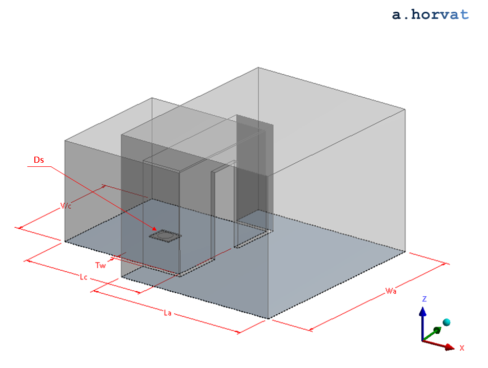
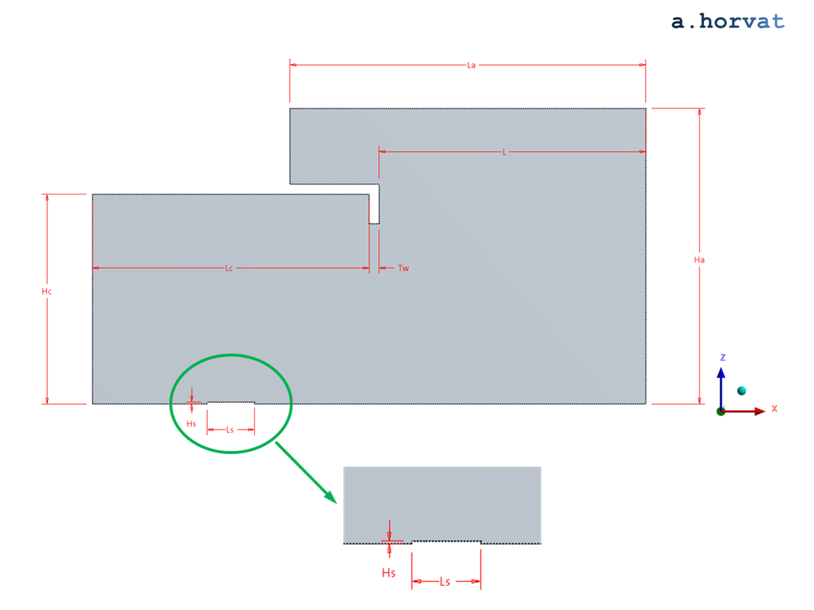
Geometry
Length, width and height of the enclosure (Lc, Wc & Hc ) are 2.8, 2.8 & 2.128 m.
Dimensions of the additional, ambient space (L, La, Wa & Ha) are 2.698, 3.6, 4.4 & 3.0 m
Wall thickness (Tw) is 0.102 m.
Fuel source is located on a square pedestal in the middle of the enclosure.
Length and width (Ls) of the pedestal are 0.42 m.
Pedestal elevation (Hs) is 0.02 m.
Fuel source diameter (Ds) is 0.3 m.
Note that small variations in the fuel source location and elevation may cause signification changes in fire behaviour
especially where the fire interacts with a boundary layer.
Loading
Fluid motion is induced by combustion of methane gas, which is introduced
to the simulation domain via a prescribed mass flow rate of a predetermined
caloric value. Three test cases [1] are analysed:
test 18: `Q_(source) = 62.9` `"kW"`
test 19: `Q_(source) = 31.6` `"kW"`
test 20: `Q_(source) = 105.3` `"kW"`
Material properties
Material properties of ideal, thermally perfect gases are used for the analysis:
CH4: `M = 16.04` `"kg"//"kmol"`, `mu = 11.1*10^(-6)` `"Pa·s"`, `lambda = 0.0343` `"W"//"mK"`
O2: `M = 31.99` `"kg"//"kmol"`, `mu = 19.2*10^(-6)` `"Pa·s"`, `lambda = 0.0266` `"W"//"mK"`
N2: `M = 28.01` `"kg"//"kmol"`, `mu = 17.7*10^(-6)` `"Pa·s"`, `lambda = 0.0259` `"W"//"mK"`
CO2: `M = 44.01` `"kg"//"kmol"`, `mu = 14.9*10^(-6)` `"Pa·s"`, `lambda = 0.0145` `"W"//"mK"`
H2O: `M = 18.02` `"kg"//"kmol"`, `mu = 9.4*10^(-6)` `"Pa·s"`, `lambda = 0.0193` `"W"//"mK"`
For the specific heat capacity, NASA SP-273 format [4] is utilised.
Thermal radiation emissivity and absorptivity of gaseous mixture is calculated using a multigrey radiation model [5].
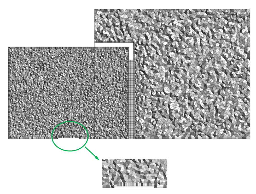
Meshing
A numerical grid with tetrahedral elements is used in all simulation cases with the element size set to 8 cm.
In the enclosure, the grid spacing is reduced to 4 cm. The grid is further refined at the surface of the fuel source,
where the grid spacing decreases to 2 cm.
Five layers of prismatic elements are used with the first layer height of 4 mm.
Cross-section of the numerical grid
The utilised numerical grid contains 0.638 mil nodes and 2.98 mil elements.
Initial conditions
Due to buoyancy induced instabilities, the system exhibits large scale transient
flow structures. For that reason, a transient CFD simulation is required.
Initially, the enclosure as well as the ambient space is occupied by air,
which is assumed to contain 21% O2 and 79% N2 by volume.
An ambient temperature (`T_(amb)`) is prescribed to the whole domain. It is 31°C for test 18,
29°C for test 19, and 35°C for test 20.
A reference pressure of 1 atm is set at the floor level of the enclosure. The vertical variation
of pressure follows the hydrostatic relationship of an incompressible fluid.
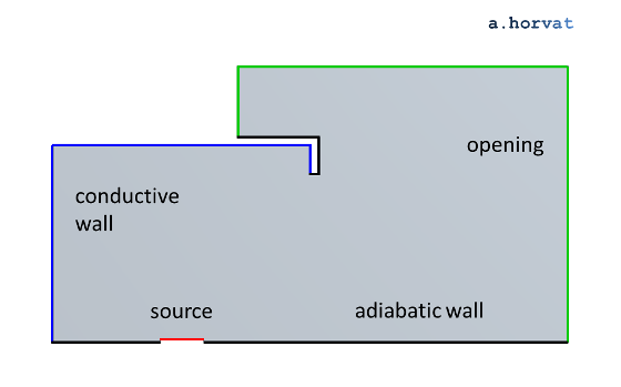
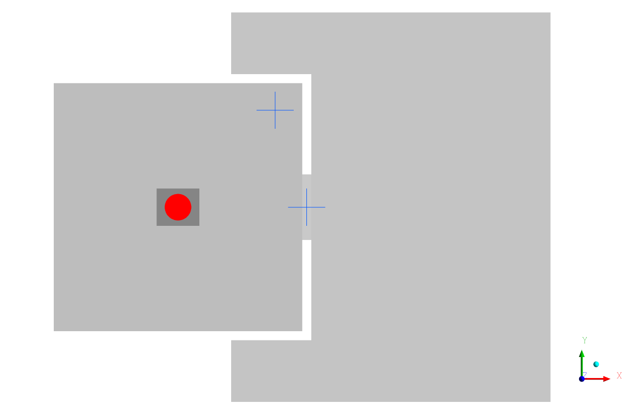
Boundary conditions
For the fuel source (marked red), the prescribed caloric value [1] has been converted
to the methane mass flow rate:
`dot(m)_(CH_4) = Q_(source)/(Delta H_(CH_4, comb)) M_(CH_4)`
For three analysed tests the following parameters are used:
test 18: `Q_(source) = 62.9` `"kW"`, `dot(m)_(CH_4) = 1.25755` `"g"//"s"`, `T_(source)=31^"o""C"`
test 19: `Q_(source) = 31.6` `"kW"`, `dot(m)_(CH_4) = 0.63176` `"g"//"s"`, `T_(source)=29^"o""C"`
test 20: `Q_(source) = 105.3` `"kW"`, `dot(m)_(CH_4) = 2.10536` `"g"//"s"`, `T_(source)=35^"o""C"`
Note that the inflow temperature (`T_(source)`) is assumed to be equal to the temperature of the ambient (`T_(amb)`).
In all case, the turbulence intensity of the inflow is set to 5% and its eddy viscosity to `10mu`.
Nevertheless, a limited sensitivity analysis has shown a negligible impact of the inflow turbulence level
on the overall results.
A substantial heat loss is assumed across the walls of the enclosure
as indicated in [2 & 3]. For that reason, the overall heat transfer
coefficient of 7 W/m2K is prescribed to the
internal, top and side surfaces of the enclosure (marked blue).
The ambient temperature (`T_(amb)`) is used as a far-field temperature;
31°C for test 18, 29°C for test 19, and 35°C for test 20.
The bottom as well as all external surfaces can be treated as adiabatic (marked black).
Opening conditions that permit inflow and outflow over the same surface are set
at the external boundaries of the ambient volume (marked green).
The hydrostatic variation of pressure is used as a pressure boundary with
the reference pressure of 1 atm at z = 0 m.
The inflow temperature of the entrained air is assumed to be equal to
the temperature of the ambient (`T_(amb)`):
31°C for test 18, 29°C for test 19, and 35°C for test 20.
Type and location of utilised boundary conditions
Results
Transient simulations were conducted using a double precision CFD solver.
For turbulence modelling, k-ε model was selected. The turbulence production term due to buoyancy:
`P_(kb) = -mu_t/(rho Sc_t) g_i del_i rho`
was included in the turbulence kinetic energy (`k`) and its dissipation rate (`epsilon`)
transport equations. The dissipation coefficient `C_3` in the epsilon transport equation was set 0.2:
`P_(epsilon b) = C_3 max(0, P_(kb))`
Figure below shows fire behaviour in the enclosure. The fire is
marked by a red isosurface of 300°C. The separation between the hot-upper
and the cold-lower layer is illustrated by a grey isosurface, which represents
a combined volume fraction of combustion products of 2.4 %.
Fire behaviour - combustion product fraction of 2.4 vol % (grey) & temperature of 300°C (red)
Vertical distributions of temperature and of flow speed are measured in the corner of the
enclosure, 0.305 m from the wall in both horizontal directions.
In addition, measurements are also taken in the middle of the door to estimate the entrainment of the ambient air [1].
Location of temperature and flow speed measurements
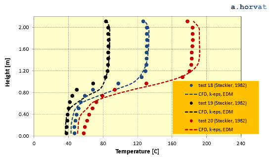
A comparison of the experimental data and the CFD simulation results is presented
below for tests 18, 19 and 20. The cumulative error of thermocouple measurements was estimated to be at least +2/-4°C [1].
Vertical distribution of temperature in the corner for tests 18, 19 & 20
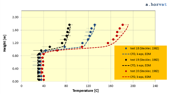
Vertical distribution of temperature across the door for tests 18, 19 & 20
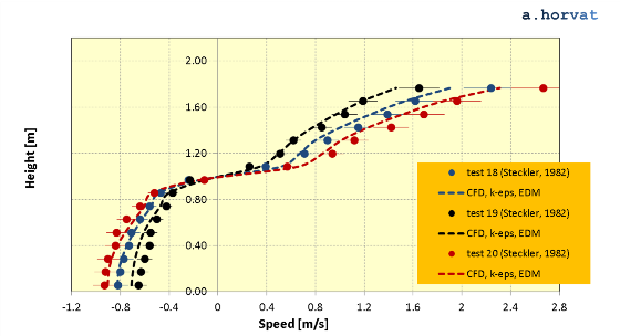
Vertical distribution of flow speed across the door for tests 18, 19 & 20
Quadratic mean (or RMS) of deviation between the experimental data [1] and the current
CFD simulation results is calculated for all three tests:
K.D. Steckler, J.G. Quintiere, W.J. Rinkinen, Flow induced by fire in a compartment, U.S. Department of Commerce, National Bureau of Standards, Centre for Fire Research, NBSIR 82-2520, 1982, Washington DC, USA.
A.J. Grandison, E.R. Galea, M.K.Patel, Fire modelling standards/benchmark: Report on SmartFire phase 2 simulations, Fire Safety Engineering Group, University of Greenwich, 2001, London, UK.
K.J. Overholt, Verification and validation of commonly used empirical correlations for fire scenarios, U.S. Department of Commerce, National Institute of Standards and Technology, NIST SP 1169, 2014, Washington DC, USA.
B.J. McBride, S. Gordon, M.A. Reno, Coefficients for calculating thermodynamic and transport properties of individual species, NASA Technical Memorandum 4513, 1993.
J.S. Truelove, HTFS Handbook: Data and reference sources on emissivity of gases, 1991.
Dr Andrei Horvat
M.Sc. Mechanical Eng.
Ph.D. Nuclear Eng.