... from an idea to superior design performance with mathematical modelling and engineering analysis ...
Convective heat transfer
Introduction
Boundary layer is the area of the viscous flow near the wall where the fluid
velocity changes from the wall velocity (which is zero for a stationary wall)
to the free stream velocity (`u_infty`). This means that friction forces that oppose
the free stream motion of the fluid are confined to a relatively thin layer.
As such, the boundary layer is characterised by large flow gradients.
Development of convective boundary layer over a flat plate is mathematically
well-defined problem for which an analytical approximation exists. The present case
describes development of the momentum as well as the thermal boundary layer over
an isothermal plate. The solution of the problem allows calculation of the wall
friction and the heat transfer between the wall and the fluid flow.
Objectives
The laminar flow case examines the extent of false, numerical diffusion associated
with discretisation of the momentum and the energy equation convection terms.
The introduced numerical error is manifested by the accelerated growth of
the momentum and thermal boundary layer, which increases the boundary
layer thickness, and reduces velocity and temperature gradients.
Deficiencies in the convection term discretisation may be also exposed as
convergence problems due to unbounded amplification of local disturbances.
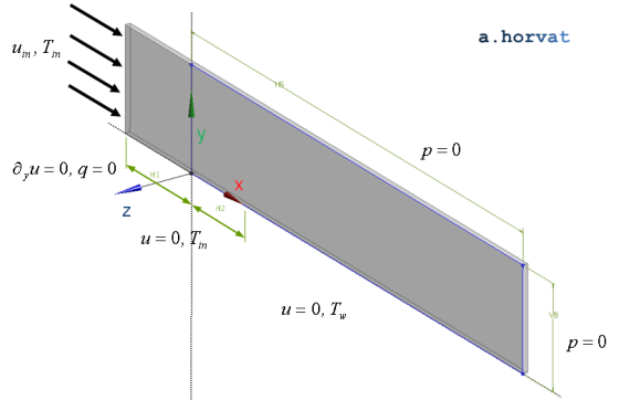
Geometry
Length of the upstream section (H1) is 2.0 m.
Length of the unheated section (H2) is 1.0 m.
Length of the momentum boundary layer development (H6) is 10.0 m.
Domain height (V8) is 2.0 m.
Domain width is 0.1 m (although not important due to the case two-dimensionality).
Loading
Uniform inflow velocity `u_(\i\n) = 1.0" m/s"` and
temperature `T_(\i\n)=20 ^" o""C"` are set for the inlet.
The momentum boundary layer develops due to the imposed no-slip wall
boundary conditions along the bottom wall.
Similarly, formation of the thermal boundary layer is initiated by
a sudden increase in the wall temperature from `T_(\i\n)=20 ^" o""C"` to `T_w=30 ^" o""C"`.
Material properties
The following fluid material properties are used:
`rho` is density of 1.0 kg/m3;
`mu` is dynamic viscosity of 0.0012 Pa s;
`c_p` is specific heat capacity of 1000.0 J/kgK;
`lambda` is thermal conductivity of 0.5 W/mK.
The fluid material properties are adjusted to yield an accelerated growth of
the momentum and the thermal boundary layer in order to avoid the need for
a very long simulation domain.
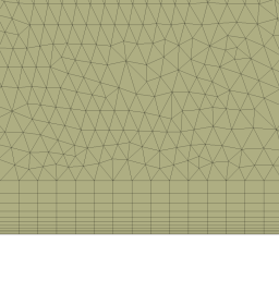
Meshing
Hexahedral grid elements are used in the simulated case. The far-field element size of 0.075 m is
refined significantly near the bottom wall to 0.004 m. In the horizontal direction, the element size is
also not uniform, but refined to 0.02 m in the area of the boundary layer trailing edge.
In the spanwise (z) direction, the 2D grid elements are extruded for a single grid spacing across the
simulation domain. a)
b)
Section of numerical grid: (a) hexahedral and (b) tetrahedral elements with the inflation layer
A numerical grid using tetrahedral mesh elements was also constructed and tested although in the two-dimensional environment
the use of flat inflation layer elements leads back to the hexahedral element form near the wall.
Initial conditions
Steady-state problem, initial conditions can be arbitrary.
Boundary conditions
Uniform velocity and the temperature at the inlet: `u_(\i\n) = 1.0" m/s"` and `T_(\i\n)=20 ^" o""C"`.
Initial section of the bottom wall (H1) with the adiabatic free-slip wall boundary conditions:
`del_y u=0.0" s"^-1` and `q=0.0" W/m"^2`.
Unheated section of the bottom wall (H2) with the no-slip boundary condition and the inflow temperature:
`u=0.0" m/s"` and `T_(\i\n)=20 ^" o""C"`.
The no-slip boundary condition `u=0.0" m/s"`, and the temperature `T_w=30 ^" o""C"` assigned to the rest
of the bottom wall (H6-H2).
For the top and the outlet boundaries, zero relative pressure is appropriate.
For the vertical X-Y surfaces, the symmetry or equivalent conditions are to be used.
Results
The exact and closed-form solution for the velocity (`u`) and the temperature
(`T`) distribution across the boundary layer does not exist. A simplified set of
fluid flow transport equations yields the Blasius solution of the boundary layer problem [1]:
`u=u_(\i\n)/2(eta f^'-f) Re_x^(-1/2)`, where `eta=y ( (rho u_(\i\n))/(mu x) )^(1/2)`,
`Re_x= (rho u_(\i\n) x)/mu`
for which `f` is obtained numerically or tabulated.
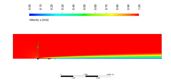
Boundary layer velocity field
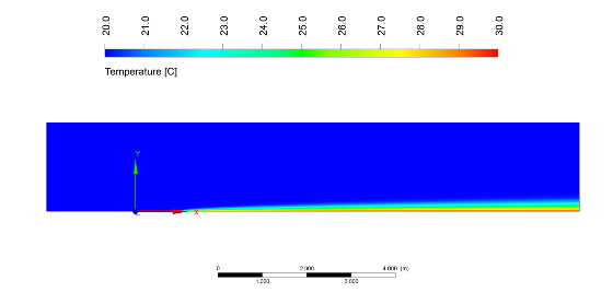
Boundary layer temperature field
A steady-state simulation was performed using a single precision CFD solver.
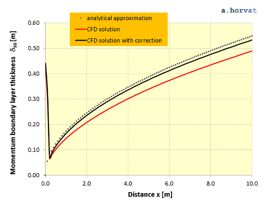
The momentum boundary layer thickness (`delta_99`), which is defined as the distance across
the boundary layer from the wall to the point where `u=0.99u_(\i\n)`, is calculated and
compared with the Blasius solution [2]:
`delta_99 / x ~~ 5.0 Re_x^(-1/2)` for `x >= 0` where `Re_x = (rho u_(\i\n) x)/mu`
Using the inlet velocity (`u_(\i\n)`) to calculate the momentum boundary layer thickness
under estimates the thickness for approximately 10% due to viscous effects and
the related flow acceleration in the far field. If the maximum velocity `u_max` at each downstream
location `x` is used to detect the velocity criterion for the boundary layer thickness, much
closer match with the Blasius solution is achieved.
Quadratic mean (or RMS) of deviation between the Blasius solution and the CFD simulation for
the momentum boundary layer thickness (`delta_99`) is 0.052 m, most of which can be attributed to the
singularity at the trailing edge.
Thickness of momentum boundary layer
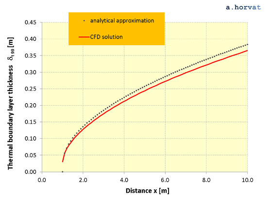
The thermal boundary layer thickness (`delta_(t 99)`) is defined as the distance across the boundary
layer from the wall to the point where `T_w-T=0.99(T_w-T_(\i\n))`. Its theoretical value is based
on the thermal boundary layer similarity solution for Prandtl numbers larger than one [4]:
`delta_(t 99) ~~ delta_99 Pr^(-1/3)` for `x-x_(\i\ni) >= 0` where `Pr = (c_p mu)/lambda`
Taking into account the unheated length of the boundary layer (`x_(\i\n)`) leads to the following expression:
`delta_(t 99) / x ~~ 5.0 Re_x^(-1/2) Pr^(-1/3) (1-(x_(\i\ni)/x)^(3/4))^(1/3)`
Quadratic mean (or RMS) of deviation between the analytical approximation and the CFD simulation for
the thermal boundary layer thickness (`delta_(t 99)`) is 0.013 m.
Thickness of thermal boundary layer
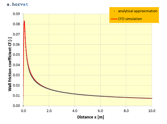
The local wall friction coefficient, which is calculated from the CFD simulation results:
`C_f = 2(mu del_y u)/(rho u_(\i\n)^2 )`
is compared with the expression derived from the Blasius solution [2]:
`C_f = 0.664 Re_x^(-1/2)` for `x >= 0` where `Re_x = (rho u_(\i\n) x)/mu`
Quadratic mean (or RMS) of deviation between the Blasius solution and the CFD simulation for
the wall friction coefficient (`C_f`) is 0.0097. Again, most of the deviation can be attributed to the
singularity at the trailing edge.
Wall friction coefficient along the boundary layer
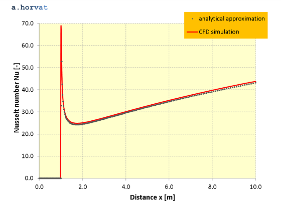
The simulation results are also used to calculate the local Nusselt number defined as
`Nu = (del_y T)/(T_w - T_(\i\n)) x`
which is compared with the expression derived from the Pohlhausen solution [3]:
`Nu = 0.332 Re_x^(1/2) Pr^(1/3) (1-(x_(\i\ni)/x)^(3/4) )^(-1/3)` for `x >= x_(\i\ni)`
Quadratic mean (or RMS) of deviation between the analytical approximation and the CFD simulation for
the wall Nusselt number (`Nu`) is 2.81.
Nusselt number coefficient along the boundary layer
 a)
a)
 b)
b)